Due December 3
Three cases are provided. The first is for a tornado outbreak in the gulf states. The 2nd is for a freezing rain event. The third is for the first round of "snowmageddon".
Use the provided maps and the web tool to analyze the events. Instructions for using the web tool are provided below. You will need to use the web tool to analyze advection, and to look at any cross sections and/or meteograms.
The links below will access the web tool for each case:
http://wx.gmu.edu/pix/case1.html
http://wx.gmu.edu/pix/case2.html
http://wx.gmu.edu/pix/case3.html
A full set of maps will be provided for each case, along with surface station plots and vertical soundings (SkewT). The links to these will be added as they become available. Return to this page and refresh your browser to see any additional links.
For Case 1:
A set of SkewT plots can be found: HERE
The station id locations for the SkewT plots are shown: HERE
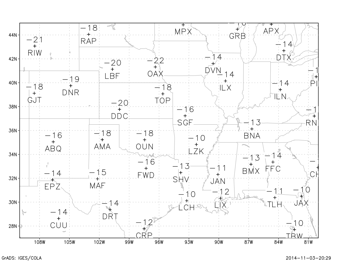
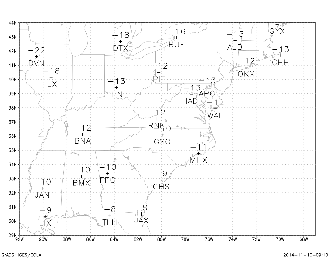
Plots of surface station data for 12Z, 18Z, and 00Z are: HERE
Satelllite photos can be found: HERE
A set of maps every six hours can be found: HERE
For Case 2:
A set of SkewT plots can be found: HERE
The station id locations for the SkewT plots are shown: HERE
A set of surface station data plots can be found: HERE
A set of maps every six hours can be found: HERE
For Case 3:
A set of SkewT plots can be found: HERE
The station id locations for the SkewT plots are shown: HERE
A set of surface station data plots can be found: HERE
A set of maps every six hours can be found: HERE
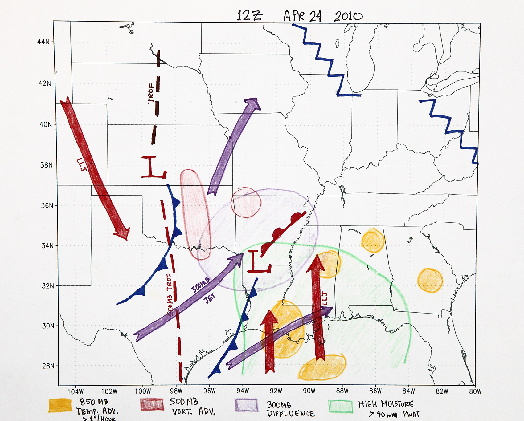
Here is an example of plotting the major features of a weather system: Click Here
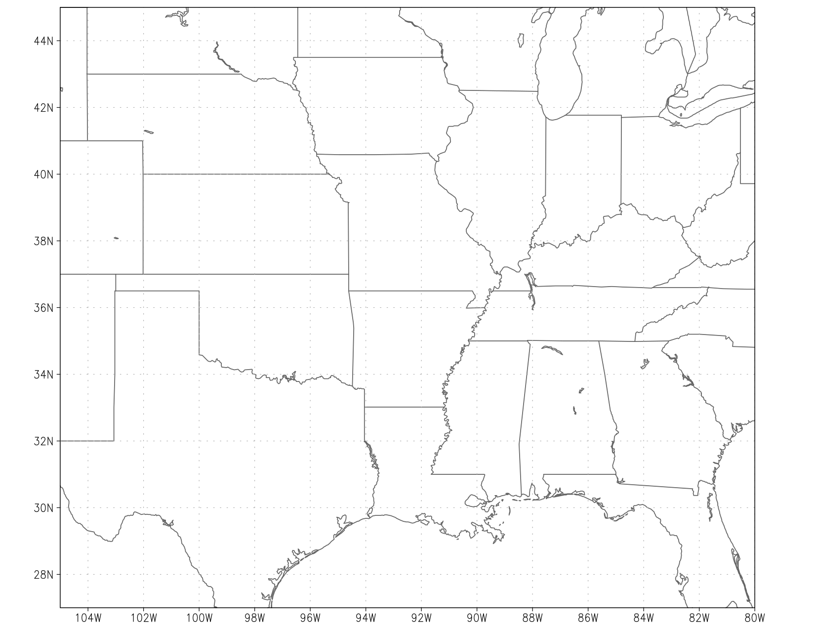
For Case 1, plot the major features on this base map: Click Here
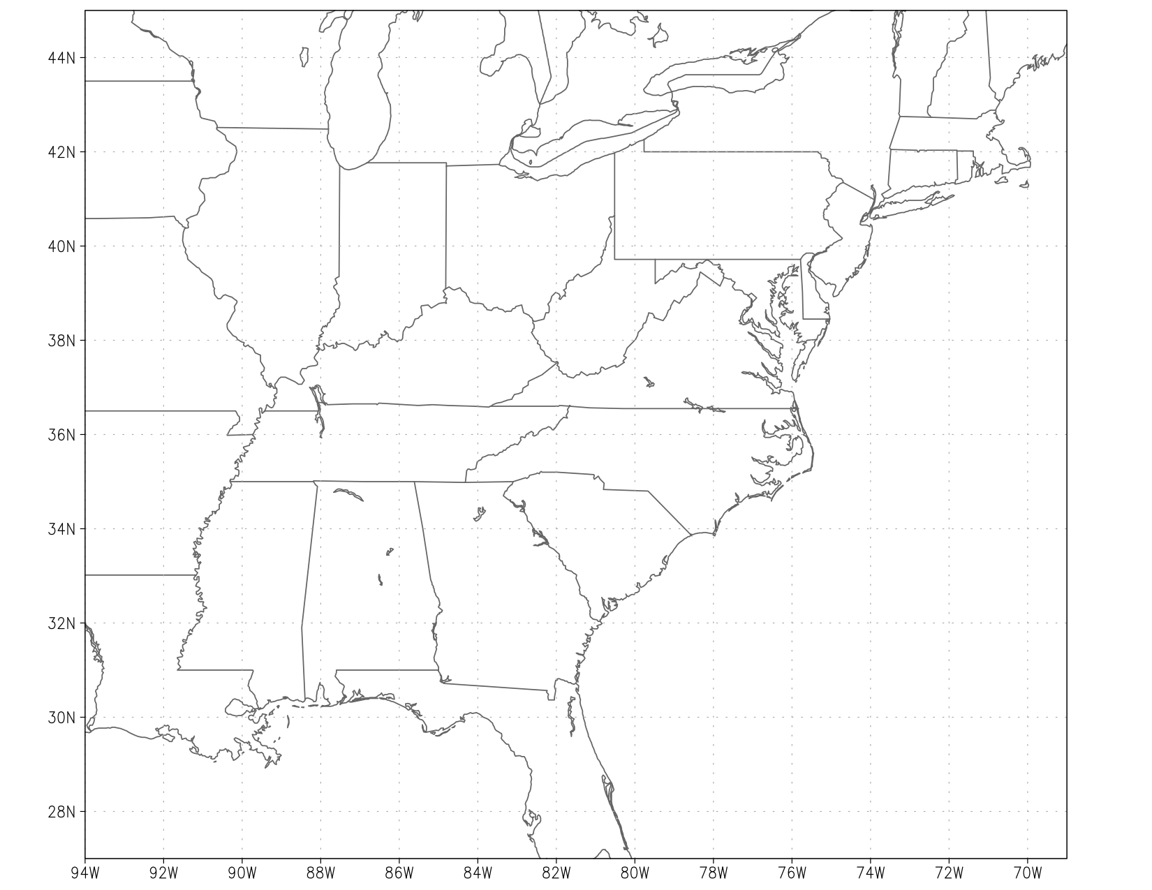
For Cases 2 and 3, plot the major features on this base map: Click Here
The features to plot are described: HERE
For Case 1, plot features at 18Z April 24, 2010 (time=23 on the web tool).
For Case 2, plot features at 00Z Dec. 9, 2013 (time=25 on the web tool).
For Case 3, plot features at 00Z Feb. 6, 2010 (time=25 on the web tool).
Note: be careful you are using the correct web tool link for each case.
In addition, answer the following questions: (tbd)
The subset of the data to view is selected using the longitude, latitude, level, and time fields. West longitude is entered as a negative value. South latitude is entered as a negative value. Time values are entered as integers. For this data set, time=1 is 00Z April 23, 2010. The data has a time interval of three hours. So time=2 would be 03Z April 23, 2010. And so on. There are 40 times in total for this data set.
The variable to be displayed is entered into the expression field. The drop-down menus can be used to obtain different mapping options. The CINT1 field can be filled in to override the default contour interval the computer selects. Once the fields have been entered, click on the Submit button to produce a plot. Note: selecting "Normal" in the "Style" drop-down menu will provide faster response time for producing plots.
The following link points to some outdated information on this interface. It also has a list of available variables from the GFS model:
Note that the variable names are arbitrary, and were selected for brevity.
Instead of just a simple variable name, math expressions can also be entered into the Expression field.
To perform addition, use the + symbol. For subtraction, use the - symbol. For multiplication, use the * symbol. For division, use the / symbol. Parentheses may be used to control the order of operation. There are a few functions also available.
Examples:
To convert Kelvin to Celsius: t - 273.15
To convert Pascals to Millibars: slp/100
To calculate the wind speed, given u and v wind components: mag(u,v)
To calculate the wind speed and convert from m/s to knots: mag(u,v)*1.94384
To calculate a time difference over three hours for some variable: z-z(t-1)
(Note: this doesn't work if time is set to 1)
To calculate a time difference over six hours for some variable: slp-slp(t-2)
(Note: this doesn't work if time is set to 1 or 2)
To calculate horizontal advection of temperature: hadv(t,u,v)
You may experiment all you like with the web tool. If you are able to break it you will get bonus points for the lab. Although, DOS attacks don't count. Please wait for your plot to appear before pressing the "submit" button again.
Here's some more information about the web tool.
The "Style" drop-down menu allows you to select the overall style of the plot. You may experiment with this, but for the lab exercises, the "Normal" setting is probably best.
There are two fields for entering expressions, Expression #1 and Expression #2. Below these two fields are some options for how to display these expressions.
The GXout1 drop down menu allows you to select how Expression #1 will be displayed:
"Default" tells the computer to try to figure
out what is best.
"Contours" tells the computer to draw Expression #1 as contour lines
"Shaded" tells the computer to draw Expression #1 as a
shaded contour plot
"Vectors" tells the computer to draw Expression #1 as wind
vectors. In this case, Expression #1 must be a compound expression.
See below.
"Stream" tells the computer to draw Expression #1 as streamlines. Again,
Expression #1 must be a compound expression.
CINT1 allows you to select a contour interval for displaying Expression #1. If you leave this field blank, the computer will select some reasonably good contour interval based on the range of the data.
The GXout2 drop down menu, and the CINT2 field, apply to the display of Expression #2, as described above.
Note that if you draw Expression #2 as a shaded contour plot, it will overlay whatever was drawn for Expression #1. This is probably a bad idea.
If you have selected the "Default" for both GXout1 and GXout2, then Expression #1 will be displayed as a colorized shaded contour plot, and Expression #2 will be displayed as black contour lines. (note that this only applies when two expressions are entered)
Similarly, if you select "Contours" for both GXout1 and GXout2, then Expression #1 will be displayed as a colorized line contour plot, and Expression #2 will be displayed as black contour lines.
So in general, the field you want to be colorized goes first, and the black overlay goes 2nd.
If you select an option to display wind data (vector or stream) you need to supply a compound expression. This is two expressions, separated by a semi-colon.
For example: u;v
If you want to colorize the vectors or streamlines based on some 3rd field, you specify that as the 3rd expression.
For example: u;v;mag(u,v)
Or perhaps: u;v;z-z(t-1)
(note: the above won't work if time is set to 1)
You may use any variable or any expression to colorize with.
If you want to draw wind arrows over a large region, you will find that there are probably too many arrows being plotted. You can use the "skip" function to reduce the number of arrows plotted.
For example: skip(u,3,3) ; v
You don't need to use the skip function twice to acheive the desired effect. In the above example, we have told the computer to only plot every 3rd arrow in both the x and y directions.
Feel free to try the above examples. Also I recomment you experiment. Try looking at various fields together. For eample, vort as Expression 1, and z as Expression 2, at the 500mb level. Or, try z-z(t-1) as Expression 1 (this gives 3 hour height change, but doesn't work if time is set to 1) and z as expression 2. Or try vort as expression 1 and slp as expression 2.