---

A Short Introduction to Numerical Weather Prediction

---

Vilhelm Bjerknes

-- Primitive Equations
-- Weather can be predicted through computation
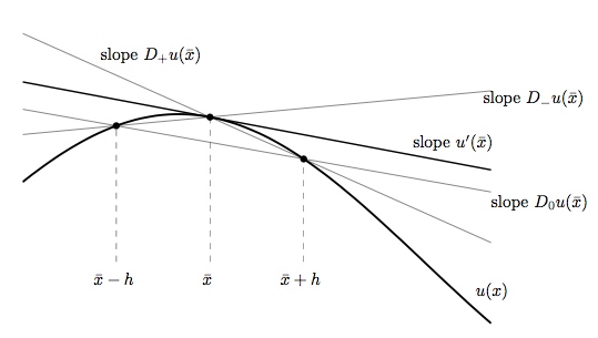
-- Graphic Calculus

Lewis Richardson

-- First attempt at Numerical Weather Prediction (1922)
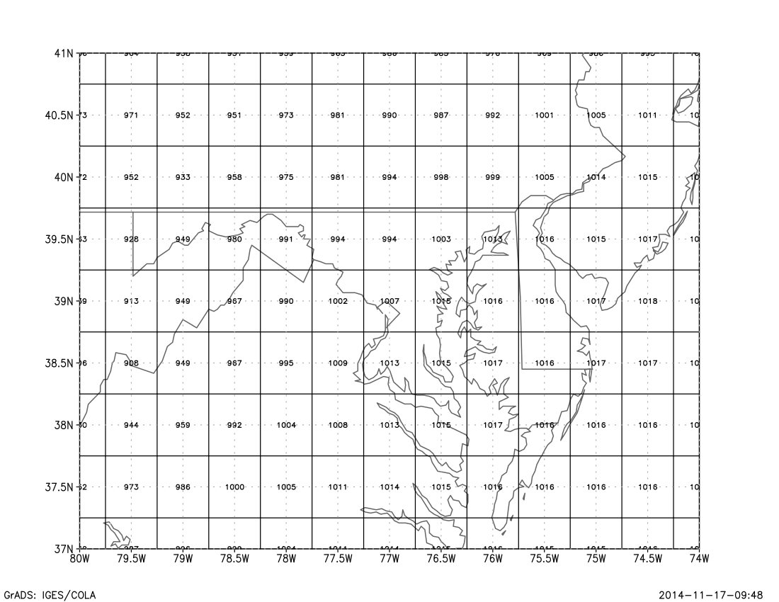
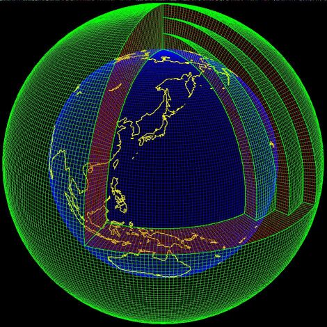
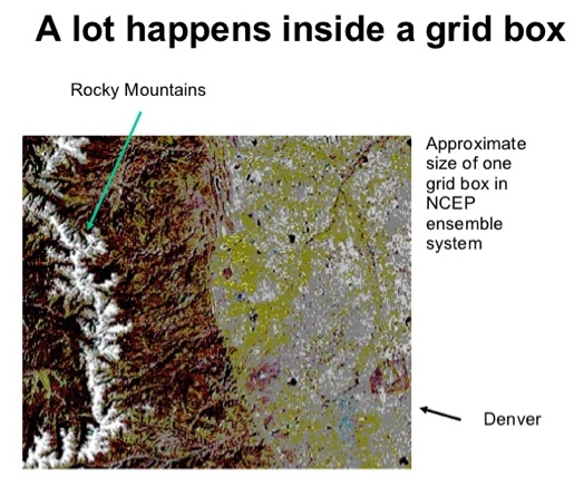
-- Technique: division of space into grid cells
-- Technique: apply finite differencing to differential equations
-- Envisioned a Forecast Factory: 64,000 people (computers) performing calculations

von Neumann and Charney (late 1940s)

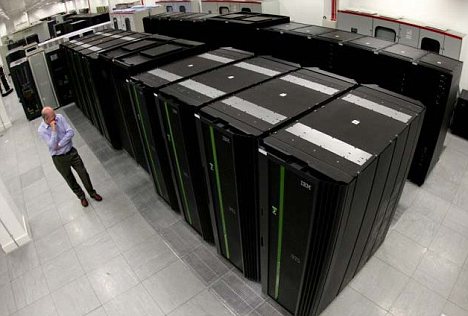
-- used ENIAC for NWP

Operational NWP

-- Barotropic models
-- Rossby and Swedish Institute of Meteorology, 1954
-- US 1955
-- (link to: History of NWP)

Primitive Equations

-- Horizontal Equations of Motion (Newton's 2nd Law)
-- Hydrostatic Equation (Vertical Stability)
-- Thermodynamic Equation (1st law of Thermodynamics)
-- Continuity Equation (Conservation of Mass)
-- Equation of State (Ideal gas properties)
-- Water Vapor Equation
-- Basic Variables: u,v,w,T,moisture
-- (link to: Primitive Equations)

Equation Simplifications

-- Barotropic
-- Quasi-Geostrophic

Solving the Equations

-- Finite Differencing (Resolution: grid spacing)
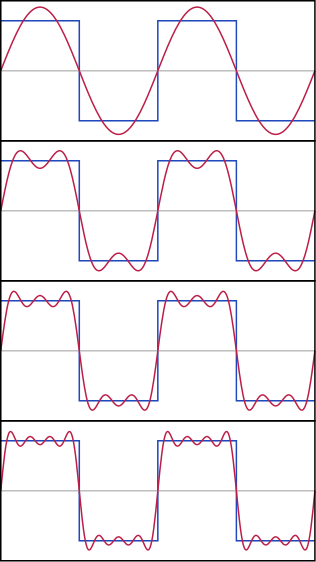
-- ... and/or Spectral (Resolution: number of coefficients)
-- Start with an initial condition
-- Step forward in time (time step)
-- Time step must be short enough for numerical stability (resolution dependent)
-- (show grads cdiff)

Initialization

-- 1950s technique: Cressman Analysis
-- Today: 4D data assimilation (GDAS)

Cressman Analysis

-- Iterative technique to get grid values from station data
-- Start with constant grid field
-- Interpolate from grid to the stations
-- Get Error: Interpolation from grid vs. actual station value
-- Apply error correction to grid values based on distance, weights, etc.
-- Repeat until error is sufficiently small
-- Hourly surface analyses on wx.gmu.edu obtained this way

Data Assimilation

-- Start with a short range forecast - "first guess"
-- Make corrections to the forecast fields to fit observations - "nudging"
-- Weed out bad data
-- Preserve interrelated physical, dynamical, and numerical consistency
-- Interpolate the data to the model grid for model initialization
-- (link: Data Assimilation)

Parameterization

-- Handle sub-grid-scale processes
-- Estimate effects of sub-grid-scale processes that cannot be directly simulated
-- Used due to lack of sufficient computing power for direct simulation
-- (link: Parameterization)

Some Processes that are Parametized

-- Land Surface
-- Cloud midro-physics
-- Turbulent Diffusion
-- Interaction with Surface
-- Orographic Drag
-- Radiative Transfer

Sources of Model Forecast Error

-- Initialization
-- Parameterization
-- Numerical approximation and truncation
-- Equation assumptions and simplifications
-- Software bugs
-- "Chaos"

Improvements to Model Forecasts

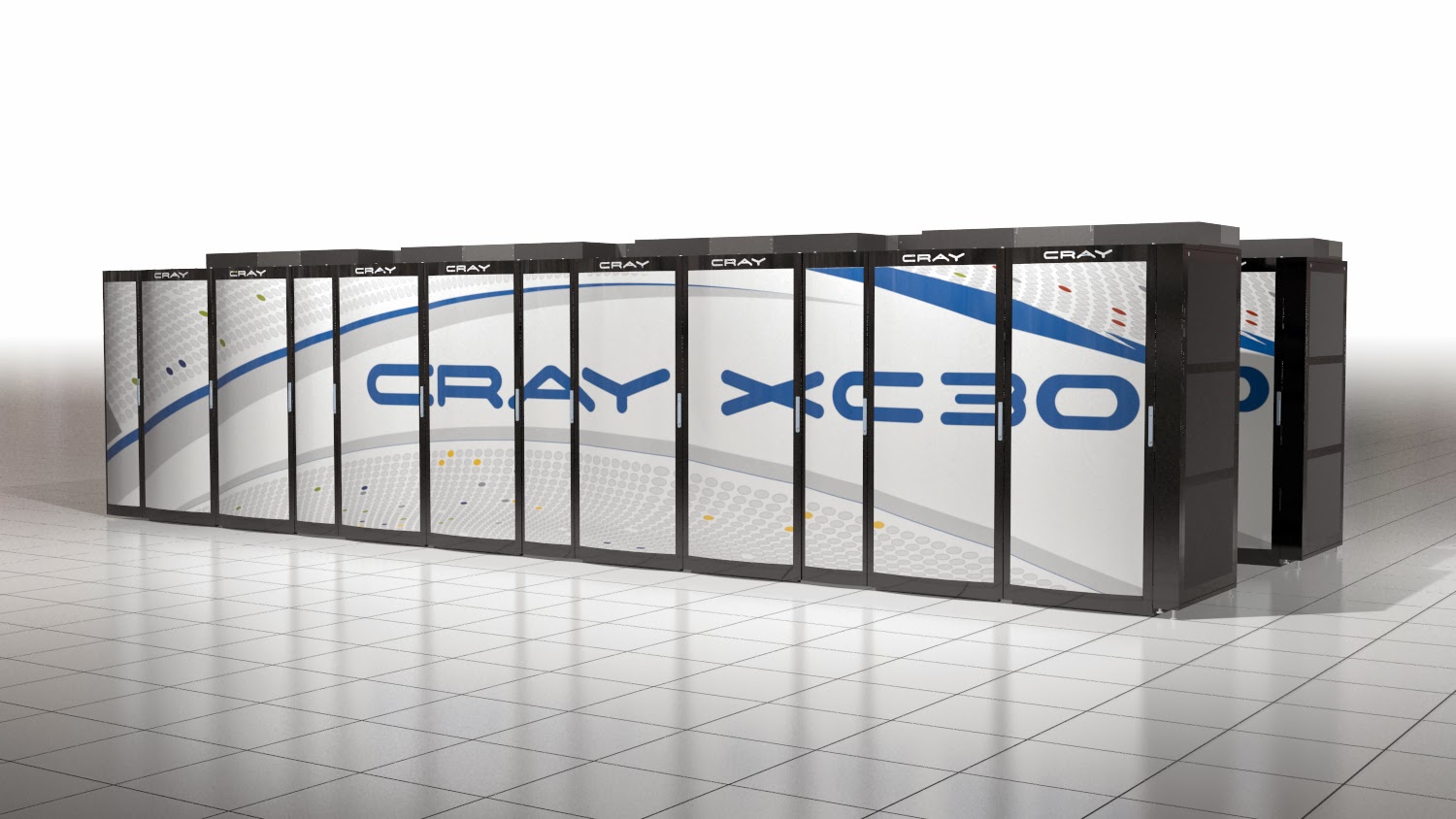
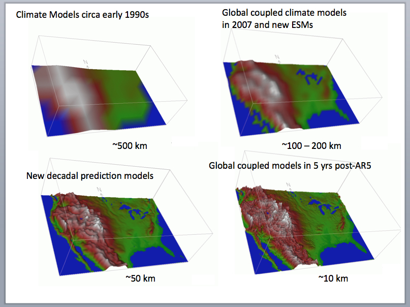
-- Faster Computers allow more complex models
-- Higher Resolution
-- Better Initialization
-- Improved numerical techniques

NCEP Models

-- (link: EMC Home Page)
-- (link: MRF Model Stats)
-- Other models

Model Output Statistics (MOS)

-- Inputs are model variables, recent obs, climatology
-- Multiple linear regression to get forecast surface variables
-- (link: Model Output Statistics)
-- (link: MOS Products)

Current Models

-- MRF: T574 (~27km), 64 Levels, time step ~2 minutes
-- We get MRF data on 0.5 degree grid
-- (link: New NWS computer)
-- (link: New MRF coming soon)
-- (link: A call for better forecasts)