You should read Chapter 3 in Vasquez, and also read the lectures notes on "Adiabatic Processes; Moisture".

Using the online tool linked HERE, you can select the different lines to become familiar with how they look.

Example 1:

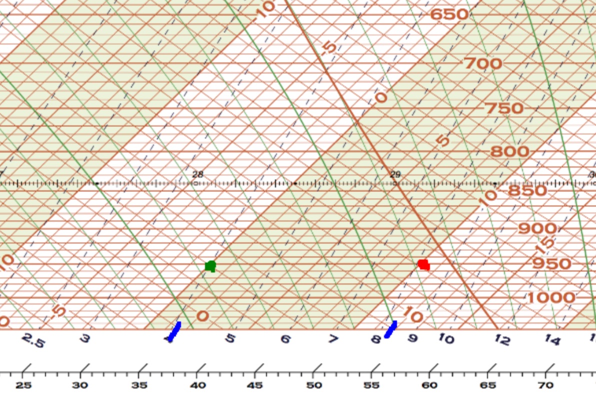
Below is an example of finding RH using the SkewT chart. The temperature of 10°C at 950mb is plotted as a red dot on the chart. The dewpoint of 0°C is plotted as a green dot on the chart.

The saturation mixing ratio at the red dot is read off the chart as about 8.2g/kg. This is the saturation mixing ratio for the parcel of air at 950mb. The saturation mixing ratio at the green dot is read off the chart as about 4.1g/kg. This is the actual mixing ratio for the air parcel at 950mb.

The RH is the ratio of these two values times 100:

RH = 100*4.1/8.2 = 50%

Example 2:

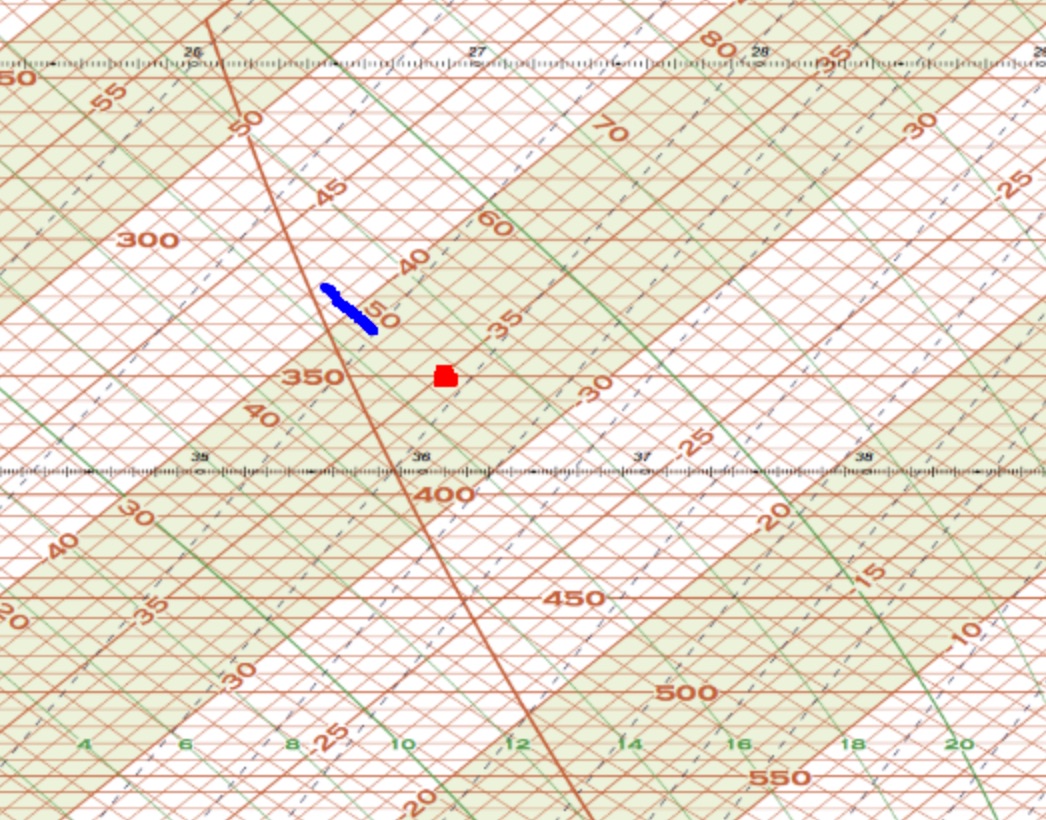
If you have a temperature and a pressure, you can find the potential temperature of that air parcel. Plot the temperature/pressure point on the SkewT and then read off the potential temperature as labeled on the dry adiabat lines.

For the example below, the temperature is -35°C and the pressure is 350mb. The dry adiabats are lines of constant θ, the blue line shows the approximate value which is about 49°C.

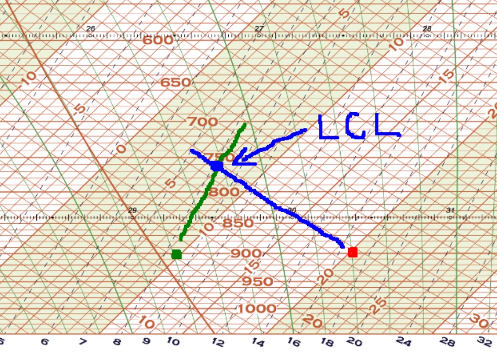
For any air parcel, if you have the pressure, temperature, and dewpoint, you can find the LCL (Lifted Condensation Level).

Lift the parcel until it is saturated. The temperature falls at the dry adiabatic rate, along a dry adiabat line. The actual mixing ratio of the parcel remains constant during a dry adiabatic process. You can find the actual mixing ratio for the parcel by using the saturation mixing ratio at the dewpoint.

In the example below, the temperature is plotted as a red dot and the dewpoint is plotted as a green dot. As the parcel ascends, the temperature drops, as the the dry adiabat is followed, and the mixing ratio stays the same. The temperature drop along the dry adiabat is shown as a blue line, and the line of constant mixing ratio is shown as a green line. When the two lines meet, the saturation mixing ratio for the parcel is the same as the actual mixing ratio for the parcel, and the parcel is saturated. This point is the LCL. Reading off the chart, the pressure at the LCL is about 760mb and the temperature at the LCL is about 7°C.

For the following examples, the full sounding is plotted on the SkewT chart. The sounding is a series of points, and the points are connected by straight lines. For the examples, a simplified SkewT chart is shown. The temperature is plotted as a red line, and the dewpoint is plotted as a green line.

Example 4:

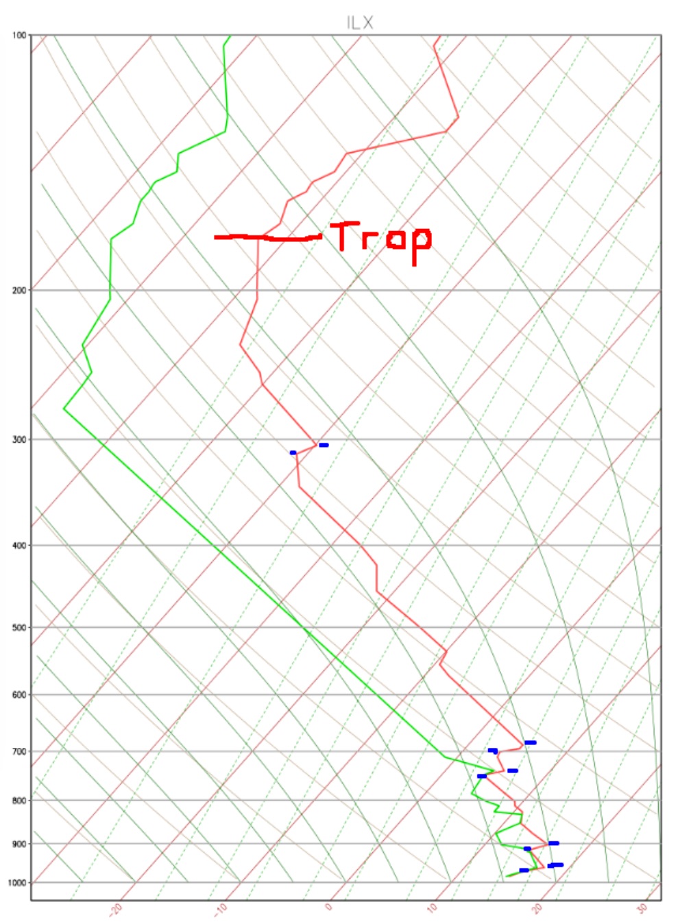
The tropopause is identified as the pressure level where the temperature stops falling with height or even starts rising with height. It is usually around 200mb. It is really more of a transition zone rather than a single level.

Between the surface and thetropopause, layers where the temperature is constant or rising with height are called inversions.

For the sounding below, the tropopause has been labeled "Trop". The inversions have been marked with small blue lines.

Example 5:

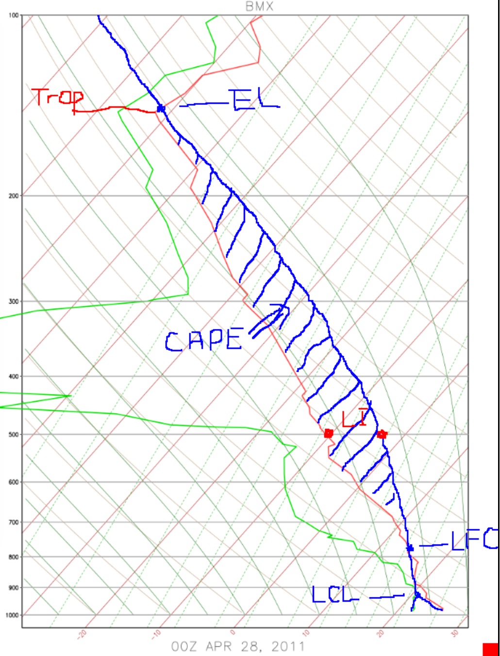
On the sounding below, the surface parcel has been lifted to the top of the chart, as indicated by the blue lines. The LCL, LFC (Level of Free Convection), and EL (Equilibrium Level) have been labeled. The positive energy area, CAPE, has been hatched with blue and labeled.

At the 500mb level, the temperature of the sounding and the temperature of the lifted surface parcel are indicated as red dots. The temperature of the sounding is about -11 and the temperature of the lifted parcel is about -3. These two temperatures are used to calculate the surface-based lifted index, which in this case is (-3) - (-11) = -8.

Not all soundings will have an LFC and an EL. All air parcels have an LCL. If the parcel is saturated before being lifted, then the LCL is at the same level as the parcel.

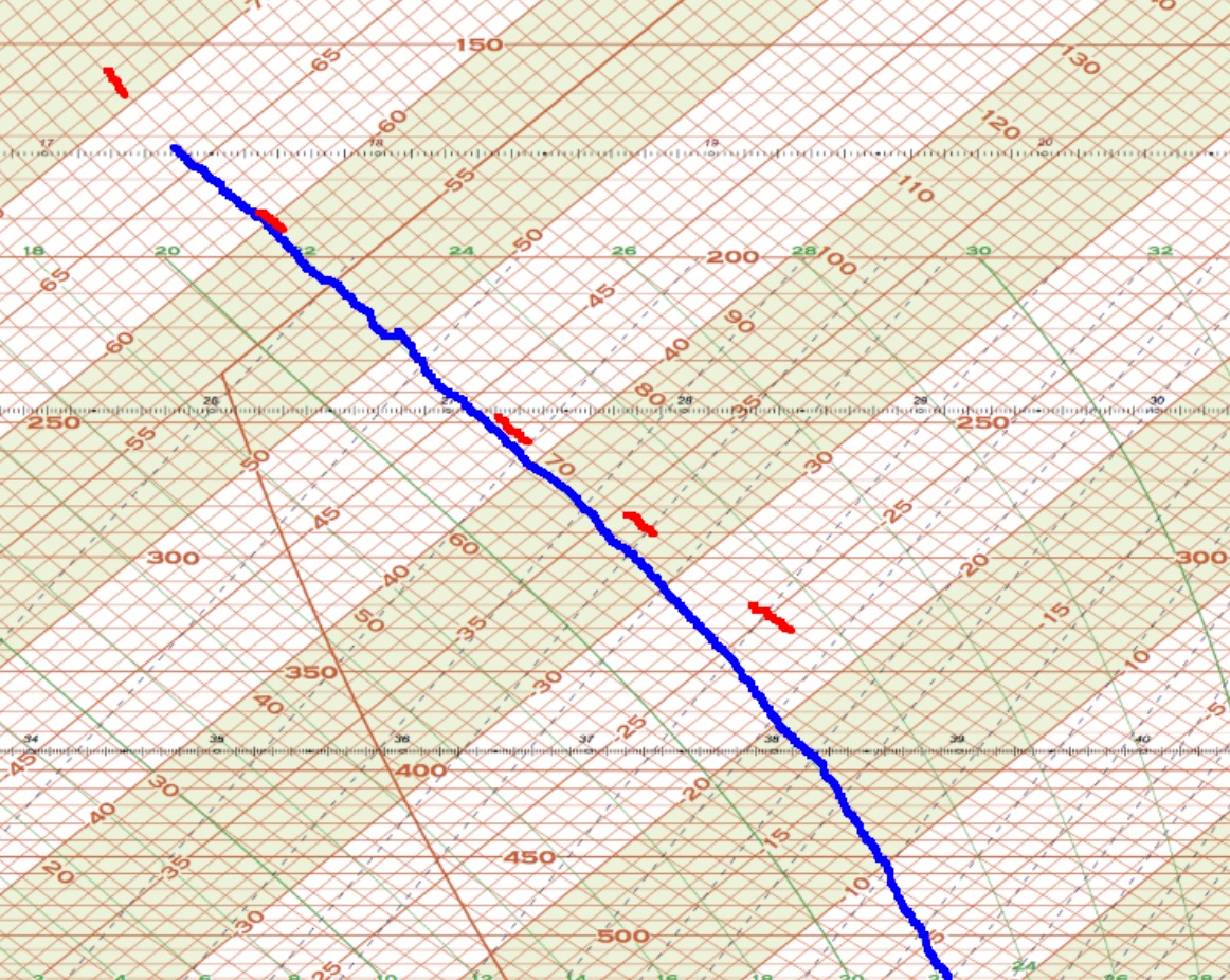
Example 6:

You can obtain the value of the equivalent potential temperature θ_e or "theta-e" for any air parcel, if you have the temperature, dewpoint, and pressure. Lift the parcel, first to its LCL, then moist adiabatically until the moisture is mostly gone from the parcel -- where the moist adiabats nearly are parallel to the dry adiabats. This will be near the top of the chart. Then read the value of the potential temperature from the dry adiabat lines.

On the example below, the top of the parcel path is shown as a blue line following the moist adiabat. The moist ascent begins to parallel the dry adiabats at about 200mb (in this portion of the chart). The parcel ends up lifting along the dry adiabat labeled with a potential temperature of 70°C. This dry adiabat is shown on the chart using short red dashes. So the θ_e of this parcel is 70°C.