The common example is that of an artillery shell fired a long distance. It will land somewhat to the right (in the northern hemisphere) of the expected path, if the coriolis force is not taken into account. Although the shell is on a ballistic arc, it appears to curve to the right to an observer on the earth's surface. It acts as though there is a force being applied to it, to the right of its movement.
The coriolis force is extremely important when considering synoptic-scale atmospheric wind flow.
It is convenient to define the coriolis parameter:
f = 2⋅Ω⋅sin(φ)
...where Ω is the earth's rotation and φ is the latitude. The earth's rotation Ω has the value 7.292 x 10⁻⁵sec-1. This is actually in radians per second, but radians are considered unitless. If you multiply by the number of seconds in a day, you get a value slightly over 2π which is the amount of rotation in a solar day (vs. the rotation in a sidereal day -- look it up if you are curious).
Using the coriolis parameter, the equations for the coriolis acceleration in terms of the component vectors (u and v) are:
Fx = f⋅v
Fy = −f⋅u
Note that the acceleration in the x direction is a function of v, and the acceleration in the y direction is a function of u.
There are a few more things to note at this point. The first is, the coriolis acceleration is a function of the speed of the object (in our case, air) and the latitude. The effect is stronger towards the poles, and weaker towards the equator. The faster the motion, the stronger the effect. An object at rest has no coriolis acceleration!
The second thing to note is, the direction of the coriolis acceleration is always to the right of the motion in the northern hemisphere.
Consider when u is zero, and v is positive -- winds from the south, towards the north. Thus we use only the first equation; Fy is zero. The acceleration is entirely in the positive x (or u) direction, which is towards the east. In other words, to the right of the motion. Thus, air moving due north will tend to curve towards the east.
Similarly, consider when v is zero and u is positive. This is a wind from the west towards the east. Thus we use only the second equation. This results in a negative acceleration in the y (or v) direction (notice the minus sign on the 2nd equation). So the wind blowing from the west will curve towards the south.
We have already discussed that when the pressure gradient is steep (the Isobars are closely spaced), the winds will be stronger. This is a result of the pressure gradient force. Intuitively, we can see that the rate of change of pressure (over some unit distance) will be proportional to the acceleration on a parcel of air.
We will consider the pressure gradient as a function of geopotential height, since that is more convenient when using upper air charts. As a function of geopotential height, the pressure gradient acceleration is the acceleration due to gravity (g) times the gradient of the geopotential height (see Wallace & Hobbs Ch. 7). As we have discussed in class, the gradient of a field is the rate of change perpendicular to the contour lines -- this is the maximum rate of change of a scaler field at a point.
Expressed mathematically, the pressure gradient force on a pressure surface can be given as the x and y components of the acceleration:
Gx = −g⋅(∂Φ/∂x)
Gy = −g⋅(∂Φ/∂y)
which can be approximated by:
Gx = −g⋅(ΔΦ/Δx)
Gy = −g⋅(ΔΦ/Δy)
where Φ is the geopotential height. The acceleration will be positive in the "downhill" direction, eg from higher heights to lower heights. Thus the minus signs in the equations. (Note these equations are approximations; the correct equations are partial differential equations.)
As an example, consider two points. At point A the geopotential height is 5000 meters. At point B the geopotential height is 5050 meters. Point B is 100km east of point A.
ΔΦ is 50 meters. Δx is 105meters. Gx = −9.8m⋅sec-2⋅50⋅10-5 = −4.9x10⁻³m⋅sec-2.
Note the negative sign indicates the acceleration is in the negative x (or u) direction, which is from the east towards the west. This makes sense, since the higher heights at point B are east of the lower heights at point A.
For a complete derivation, see Wallace & Hobbs Chapter 7 through page 281.
Consider an air parcel at rest but under acceleration due to a pressure gradient force. It will begin moving in the "downhill" direction of the pressure gradient. However, once it begins moving, it will begin to turn to the right, due to the coriolis acceleration.
Hmmmm.
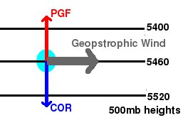
As it begins turning right, the parcel's motion will become oriented such that higher pressures (or heights) are to the right, and lower pressures are to the left. If no other forces are involved, at some point the parcel will achieve a motion where there is a balance between the pressure gradient force and the coriolis force. This balance is called the geostrophic balance and the motion required to acheive that balance is called the geostrophic wind. For large scale flow in the upper atomosphere, the pressure gradient force and the coriolis force are the largest forces acting on the air, so the winds tend to be within about 10% of geostrophic balance.
The component equations for the geostrophic wind are:
ug⋅f = −g⋅(∂Φ/∂y)
vg⋅f = g⋅(∂Φ/∂x)
This can be approximated by:
ug⋅f = −g⋅(ΔΦ/Δy)
vg⋅f = g⋅(ΔΦ/Δx)
These equations express the balance between the coriolis force (on the left side of the equation) and the pressure gradient force (on the right side of the equation). To solve for the u and v components of the geostrophic wind (denoted by the g subscript), we divide both sides by the coriolis parameter f.
Here is an idealized diagram of the geostrophic wind:
Let's do an example. If the change of height is constant from 30N to 40N and it drops 40 meters per degree of latitude (so it drops 400 meters from 30N to 40N), how strong is the geostrophic wind at 35N? Assume there is no change of height in the longitude direction.
Solution:
In this case we have a change of height in y (latitude) but no change in x (longitude). So we will use the first equation above and solve for ug. (If heights were only changing in the x direction, we would use the 2nd equation above and solve for vg. If both x and y are changing, we would need to use both equations.)
The coriolis parameter at 35N is 2 ⋅ Ω ⋅ sin(35°) = 2 ⋅ 7.292x10-5sec-1 ⋅ 0.5736 = 8.36x10⁻⁵ sec-1
g/f = 9.8m⋅sec-2 / 8.36x10⁻⁵ sec-1 = 1.17x10⁵m⋅sec-1
ΔΦ = −40 meters and Δy = 1° Latitude = 1.11x10⁵ meters
Note that the height is dropping (negative change) as y (latitude) is increasing. Thus the negative sign on Δφ. This cancels the negative sign in the equation.
So this gives us 1.17x10⁵m⋅sec-1 ⋅ 40 meters / 1.11x10⁵meters
which calculates to 42.16⋅m⋅sec-1. This is a postive u component wind, so it is blowing from west to east.
Converting to knots by multiplying by 1.93, we get a geostrophic wind speed of 81.4 knots.
To calculate the distance when both longitude and latitude are changing is complex. We avoid this issue by working with the vector components, which allows us to deal only with the cases where longitude varies and latitude is fixed, or where latitude varies and longitude is fixed.
If we want to work with data that is in spherical (latitude-longitude) coordinates we need to adjust for that. With λ for longitude and φ for latitude, r for the radius of the earth, the equations for the u and v components of the geostrophic wind are:
ug = −(g/f)⋅(1/r)⋅(∂Φ/∂φ)
vg = (g/f)⋅(1/r⋅cosφ)⋅(∂Φ/∂λ)
Below is a plot of the 500mb level, showing the heights and winds from model initial conditions. In addition, an estimate of the geostrophic winds are plotted as green wind arrows. Note that there are, in some places, fairly large differences between the two fields. These differences are called ageostrophic winds.
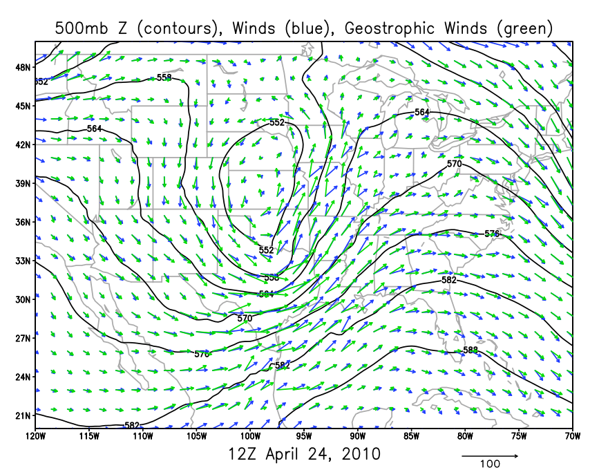
The estimate of the geostrophic wind shown above was obtained using a technique called finite differencing. This is a common way of doing calculations on a weather map for diagnostic use. In the next lecture, we will start with an example of using finite differencing to obtain the geostrophic wind.