The difference between geostrophic wind at a point and the observed wind at that point is called the ageostrophic component of the wind. An observed wind that is slower than the geostrophic wind at a point is called subgeostrophic. An observed wind that is faster than the geostrophic wind at a point is called supergeostrophic.
In the last lecture, we discussed the equations for the geostrophic wind. These equations were presented in component form, where the u and v components of the geostrophic wind could be determined separately. Once one has the u and v components, the direction and speed can be determined.
If we combine the two component equations, we can determine the speed of the geostrophic wind based on the gradient of the geopotential height. Remember the gradient is the change of height along a direction perpendicular to the contours. (For those who have taken the third semester of calculus, the gradient is the del operator on f(x,y)).
The equation is:
wsg = (g/f)⋅ΔΦ/Δd
where wsg is the geostrophic wind speed, and d is the distance along the gradient direction. Here we are taking the change of Φ in the direction of the gradient. Note again that this equation is an estimate of the geostrophic wind speed -- the true equation expresses the rates of change in the infinitesimals of the calculus.
The calculation of the estimated geostrophic wind speed is similar to the example shown in the previous lecture. But instead of calculating the rate of change of heights in a north-south direction, as shown in the example, we calculate the rate of change of heights in the direction of the gradient. And since we are only calculating wind speed, we can take the absolute value of the quantities (and not worry about the direction of the gradient).
However, we observe curved wind flow all the time, such as the wind flowing around highs and lows, and through troughs and ridges. For the wind to follow a curved path, the wind is not in geostrophic balance.
For wind to travel in a cyclonic curved path, it curves to the left of straight line motion. This requires that the pressure gradient force be stronger than the coriolis force. For this to happen, the wind velocity must be less than geostrophic (remember that the coriolis force is propotional to wind velocity). Thus cyclonic curved winds are subgeostrophic.
Winds that have anticyclonic curvature curve to the right of straight line motion. Thus the coriolis force must be stronger than the pressure gradient force. For this to be the case, the wind velocity is greater than the geostrophic wind speed, so the winds are supergeostrophic.
So for an anti-cyclone, or a ridge, it is the coriolis force that is causing the acceleration and rotation. So the strength of an anti-cyclone is limited by the coriolis force. There is no such limit for a cyclone, since there is no real limit to the strength of the pressure gradient force. This is the main reason why the center of a high will be broad and flat, where the center of a low is often fairly tight, with strong pressure gradients.
The balance of forces that results in a wind blowing parallel to curved isobars or height contours is called the gradient wind balance.
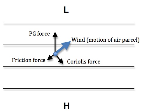
Friction is a force that acts in the direction opposite the wind direction. This results in the wind slowing to be subgeostrophic, which results in less coriolis force. When a balance of forces is obtained, this is what it looks like:
The wind crosses the isobars from higher to lower pressure. This is commonly seen on surface maps.
Mathematically, we think of the wind as a vector, and the property being advected as a scalar. The advection is the rate of change of the scalar property with time at a point. This rate of change is determined by the wind speed, and the horizontal rate of change of the scalar in the direction of the wind.
For example, if the wind is blowing at high speed across a dense packing of isotherms, the temperature advection would be strong, eg the rate of change of temperature would be rapid at a fixed point within the dense packing of isotherms.
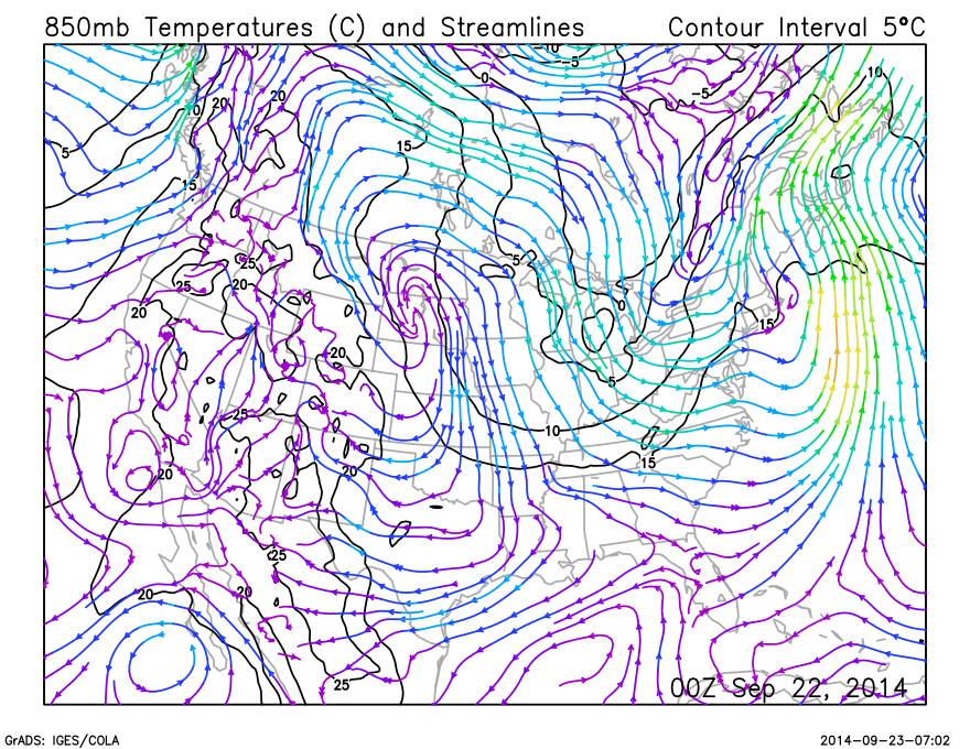
One way to determine advection on a weather map is to plot contours of a scalar quantity such as temperature, then overlay streamlines that are colorized by speed. This is difficult to do by hand, but the computer can easily produce such a plot, for example:
An estimate of horizontal advection can also be calculated using finite differencing, when gridded data is available.
You will see the abbreviation CAA used to mean Cold Air Advection, and the abbreviation WAA used to mean Warm Air Advection.
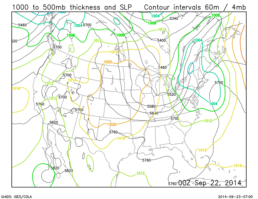
If we plot some sort of scalar quantity such as temperature, using contours, and then overlay a plot of isobars or heights, we can visually determine the strength of the advection.
Where these lines cross, they form closed four sided polygons. The smaller the polygon, the stronger the advection.
Take temperature, for example. When we plot isotherms, the horizontal rate of change of temperature is highest where the isotherms are most closely spaced. And, when we plot height contours, the wind speed is highest where the contours are more closely spaced. If these two sets of closely spaced contours cross at right angles, the advection is very strong indeed!
Note the following example. It is common to plot the surface isobars along with the 1000mb to 500mb thickness, so that bulk temperature advection can be easily observed on the map.